Performance Python
This is an extension of the original article written by Prabhu Ramachandran. The original article can be found here. An addition to this article written by Travis Oliphant can be found at blogspot.com.
A beginners guide to using Python for performance computing
A comparison of weave with NumPy, Cython, opencl, and CLyther for solving Laplace’s equation. laplace.py is The complete Python code discussed below. The source tarball ( perfpy_clyther.tgz. ) contains in addition the Fortran code, the pure C++ code, the Pyrex sources and clyther functions. and a setup.py script to build the f2py and Pyrex module.
Introduction
This is a simple introductory document to using Python for performance computing. We’ll use NumPy, SciPy’s weave (using both weave.blitz and weave.inline) and Pyrex. We will also show how to use f2py to wrap a Fortran subroutine and call it from within Python. We will also use this opportunity to benchmark the various ways to solve a particular numerical problem in Python and compare them to an implementation of the algorithm in C++.
Problem description
The example we will consider is a very simple (read, trivial) case of solving the 2D Laplace equation using an iterative finite difference scheme (four point averaging, Gauss-Seidel or Gauss-Jordan). The formal specification of the problem is as follows. We are required to solve for some unknown function u(x,y) such that 2u = 0 with a boundary condition specified. For convenience the domain of interest is considered to be a rectangle and the boundary values at the sides of this rectangle are given.
It can be shown that this problem can be solved using a simple four point averaging scheme as follows. Discretise the domain into an (nx x ny) grid of points. Then the function u can be represented as a 2 dimensional array - u(nx, ny). The values of u along the sides of the rectangle are given. The solution can be obtained by iterating in the following manner:
def time_step(u, dy, dy):

    nx = u.shape[0]
    ny = u.shape[1]

    for i in range(1, nx-1):
        for j in range(1, ny-1):
            u[i,j] = ((u[i-1, j] + u[i+1, j])*dy**2 +
                      (u[i, j-1] + u[i, j+1])*dx**2)/(2.0*(dx**2 + dy**2))
OpenCL
OpenCL has two different models for parallelization, task and data parallel programming models.
- Task Parallel Programming Model:
- A programming model in which computations are expressed in terms of multiple concurrent tasks where a task is a kernel executing in a single work-group of size one. The concurrent tasks can be running different kernels
- Data Parallel Programming Model:
- Traditionally, this term refers to a programming model where concurrency is expressed as instructions from a single program applied to multiple elements within a set of data structures. The term has been generalized in OpenCL to refer to a model wherein a set of instructions from a single program are applied concurrently to each point within an abstract domain of indices.
In this article I will explore both.
CLyther
See the clyther.array.CLArrayContext for a complete overview. Since OpenCL has the idea of a Context
The environment within which the kernels execute and the domain in which synchronization and memory management is defined. The context includes a set of devices, the memory accessible to those devices, the corresponding memory properties and one or more command-queues used to schedule execution of a kernel(s) or operations on memory objects.
CLyther takes this concept of a context as an environment and uses it to mock the numpy module namespace.
In numpy to create an array you may do:
import numpy as np

a = np.arrange(100, dtype='f')
In CLyther
from clyther.array import CLArrayContext
import opencl as cl
ca = CLArrayContext(device_type=cl.Device.GPU)

a = ca.arrange(100, ctype='f')
You will notice that the preamble is longer but this is because with OpenCL we are allowed to choose which device(s) we want to run on. In this case a is a buffer of 100 floats allocated on the GPU.
Task Parallel Solution
Task Parallel:
@cly.task
def cly_time_step_task(u, dy2, dx2, dnr_inv):

    nx = u.shape[0]
    ny = u.shape[1]

    for i in range(1, nx - 1):
        for j in range(1, ny - 1):
            u[i, j] = ((u[i - 1, j] + u[i + 1, j]) * dy2 +
                      (u[i, j - 1] + u[i, j + 1]) * dx2) * dnr_inv
The clyther.task decorator adds an arguement to the function signature cly_time_step_task(queue, u, dy2, dx2, dnr_inv). In this case queue can be the attribute ca.queue.
This solution is different than cython for two reasons:
- This function is created inline in python with pure python code.
- The typing is dynamic just like python. This function can and will be specialized for the types of arguments passed to it.
Note
The argument u can also be a numpy array.
For any device in ca.devices if device.host_unified_memory == True (i.e device_type=CPU) then this will not come at any added cost.
Note
If you take a look at the results, this runs only slightly slower than the weave-fast-inline example.
In the next version I would also like to test out some optimization decorators like:
@cly.constants(['dy2', 'dx2', 'dnr_inv', ('shape', 'u')])
@cly.compile_flags(['-cl-mad-enable', ..., etc])
Data Parallel Solution
Data Parallel:
@cly.global_work_size(lambda u: [u.shape[0] - 2])
@cly.kernel
def lp2dstep(u, dx2, dy2, dnr_inv, stidx):
    i = clrt.get_global_id(0) + 1

    ny = u.shape[1]

    for j in range(1 + ((i + stidx) % 2), ny - 1, 2):
        u[j, i] = ((u[j - 1, i] + u[j + 1, i]) * dy2 +
                   (u[j, i - 1] + u[j, i + 1]) * dx2) * dnr_inv
In the this solution you will notice the following changes.
- The clyther.kernel is now clyther.kernel:
- This tells CLyther that the lp2dstep function will now run in data-parallel mode.
- The outer loop has been removed:
- You will noticed that the outer loop has been replaced by the decorator @cly.global_work_size(lambda u: [u.shape[0] - 2]) and the index i = clrt.get_global_id(0) + 1. This is telling OpenCL to run the lp2dstep in parallel for each point on an [u.shape[0] - 2] shaped grid. The indexing call clrt.get_global_id retrieves the grid-point simulating the loop index i.
- The inner loop has been changed:
The algorithm now uses a checker-board pattern for parallel data-access. I have added the argument stidx which may be 1 or 2 to compute odd or even columns respectively. this function must be called twice:
lp2dstep(ca.queue, u, dx2, dy2, dnr_inv, 1)
lp2dstep(ca.queue, u, dx2, dy2, dnr_inv, 2)
Performance Results
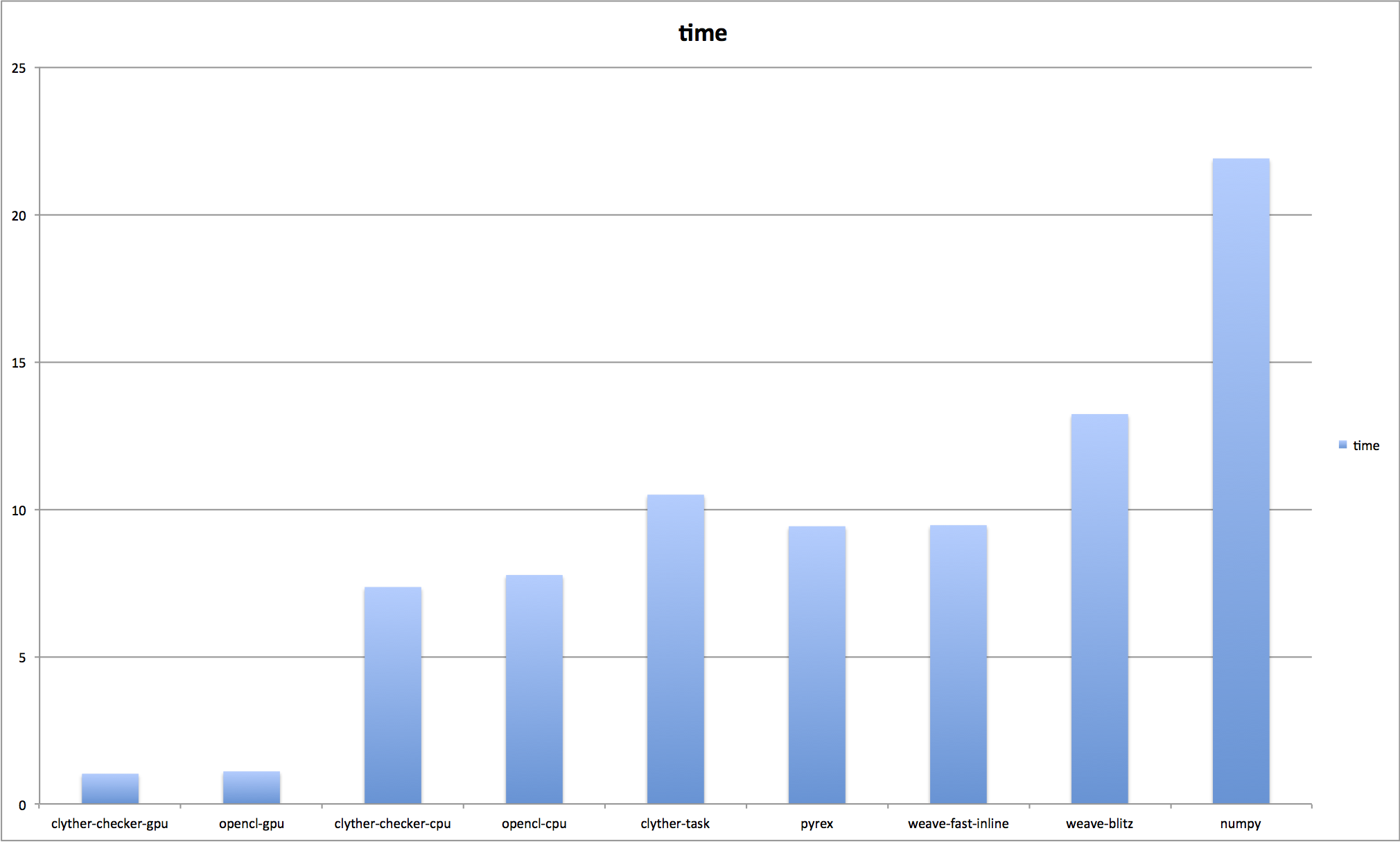
Here are the performance results.
| method | time |
|---|---|
| clyther-checker-gpu | 1.03 |
| opencl-gpu | 1.10 |
| clyther-checker-cpu | 7.36 |
| opencl-cpu | 7.76 |
| clyther-task | 10.49 |
| pyrex | 9.42 |
| weave-fast-inline | 9.46 |
| weave-blitz | 13.22 |
| numpy | 21.90 |